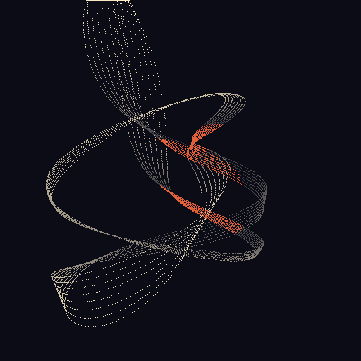
akten_quayola · Lissajous3D
Lissajous 3D
A three-dimensional Lissajous figure rendered as a single precision line drawing on a deep field. The classical parametric form x=sin(a t + δ), y=sin(b t) is extended with z=sin(c t + ε); Quayola's Lissajous series pushes these classic curves into the third dimension and prints them at architectural scale. Here, the integer frequency ratios slowly drift through random walks so the curve is never quite periodic, and a rotating perspective projection produces a sweeping, knotted figure.
Original: https://quayola.com/
▶ Try the live demo (JS port) ▶ Run reference.py via Pyodide 10 formulas have instant JS ports. The Pyodide path runs the actual Python in your browser — first load is ~6 MB, then instant.
Math essence
t.linspace(t0, t0 + 4π, N). x = ax*sin(fx_d*t + phase_xy), y = by*sin(fy_d*t), z = cz*sin(fz_d*t + phase_xz). Rotate (x, z) by angle = 0.6 + 0.25*sin(t*0.1) and perspective project: u = x/(fov + z), v = y/(fov + z). fx_d, fy_d, fz_d perform random walks to mutate the figure.
Parameters
| Name | Type | Default | Range | Description |
|---|---|---|---|---|
num_points | int | 12000 | 4000–40000 | Samples along the parametric curve. |
dim | int | 512 | 256–1024 | Output canvas side length. |
fx | int | 3 | 1–8 | Initial x-frequency integer. |
fy | int | 2 | 1–8 | Initial y-frequency integer. |
fz | int | 5 | 1–8 | Initial z-frequency integer. |
ax | float | 1 | 0.4–1.6 | Amplitude of x oscillation. |
by | float | 0.8 | 0.4–1.6 | Amplitude of y oscillation. |
cz | float | 0.6 | 0.4–1.6 | Amplitude of z oscillation. |
phase_xy | float | 0 | 0–6.283 | Phase offset for the x oscillation. |
phase_xz | float | 0 | 0–6.283 | Phase offset for the z oscillation. |
drift | float | 0.0008 | 0–0.005 | Per-step random walk magnitude for each frequency. |
fov | float | 1.6 | 0.8–3 | Perspective field-of-view divisor. |
Reference
First 60 lines of reference.py. Full source:
library_external/akten_quayola/Lissajous3D/reference.py
from __future__ import annotations

from typing import ClassVar

import numpy as np


class Lissajous3D:
    """Lissajous 3D — Quayola, *Lissajous* series (ongoing).

    Quayola's Lissajous pieces push the classical x = A sin(at + δ),
    y = B sin(bt) parametric curve out into three dimensions:
    ``x = A sin(a t + δ)``, ``y = B sin(b t)``, ``z = C sin(c t + ε)``.

    Each formula below adds a slowly evolving perturbation to the
    integer frequency ratios so the curve never quite closes; the
    rendered figure rotates around a vertical axis and is projected
    onto a 2D canvas using a simple perspective divide.  Brightness
    comes from a depth-faded ink palette, evoking the precision
    line-art feel of Quayola's plotter output.
    """

    family: ClassVar[str] = "akten_quayola"
    sketch: ClassVar[str] = "Lissajous3D"

    def __init__(
        self,
        num_points: int = 12000,
        dim: int = 512,
        fx: int = 3,
        fy: int = 2,
        fz: int = 5,
        ax: float = 1.0,
        by: float = 0.8,
        cz: float = 0.6,
        phase_xy: float = 0.0,
        phase_xz: float = 0.0,
        drift: float = 0.0008,
        fov: float = 1.6,
        background: tuple[int, int, int] = (12, 12, 22),
        **_,
    ) -> None:
        self.num_points = int(num_points)
        self.dim = int(dim)
        self.fx = int(fx)
        self.fy = int(fy)
        self.fz = int(fz)
        self.ax = float(ax)
        self.by = float(by)
        self.cz = float(cz)
        self.phase_xy = float(phase_xy)
        self.phase_xz = float(phase_xz)
        self.drift = float(drift)
        self.fov = float(fov)
        self.bg_color = np.array(background, dtype=np.float32)
        self.reset(seed=None)

    def reset(self, seed: int | None = None) -> None:
        self.rng = np.random.default_rng(seed)
        self.t = 0.0
Try running it locally
The reference implementation is self-contained Python with numpy. Install the package and run:
python library_external/akten_quayola/Lissajous3D/reference.pyNeed help? See Learn for the standard environment setup, or Playground for an in-browser sketchbook.
More from akten × quayola
Gesture Driven Field
akten_quayola · GestureDrivenField
Particles advected through a vector field whose structure is driven by a synthetic gesture signal: a chain of sinusoids at integer-related frequencies.
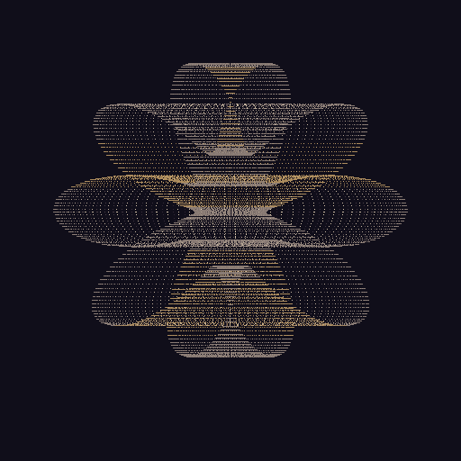
Mechanical Flower Spline
akten_quayola · MechanicalFlowerSpline
A 2D petal-radius spline r(θ) = r0 + A*cos(p*θ + δ) + B*cos(q*θ) swept 360° around a vertical Y axis to form a procedural flower-like 3D surface, then orthographically projected and depth-shaded.

Pleated Fabric
akten_quayola · PleatedFabric
A textile grid whose vertical coordinate follows z = A * envelope(y) * sin(2π f x + phase(t)), projected obliquely onto a 2D canvas so the folds read as parallel ridges of light.
Simple Harmonic Motion
akten_quayola · SimpleHarmonicMotion
A 100x100 grid of damped harmonic oscillators driven by a periodic central impulse.
Strata Landscape
akten_quayola · StrataLandscape
A geological landscape rendered as N horizontal strata stacked vertically, each band displaced by a slowly growing sinusoid and shaded with its own hue.
Wave Interference
akten_quayola · WaveInterference
N drifting point sources emit circular sinusoidal waves whose superposition is tone-mapped into a stormy ocean-like field.