generative_pioneers · haeberli_painterly
Paint by Numbers (Haeberli)
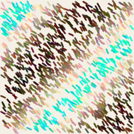
Paul Haeberli's 1990 SIGGRAPH 'Paint by Numbers' — the founding paper of stroke-based rendering. A continuous-valued target field (here one of four analytic color fields: diagonal_band, sunset, rose, valley) supplies a luminance image; N random strokes are placed uniformly across the canvas, each is assigned the local color and a local-gradient direction (with a small random jitter), and crucially the strokes are sorted by luminance and drawn back-to-front in increasing order. The result is the classic 'painterly' impressionist render: bright strokes land last and pop, dim strokes land first and recede. The simple ordering trick is the algorithmic kernel that has dominated the SBR family ever since.
Original: https://www.dgp.toronto.edu/~hertzman/sbr02/hertzmann-cga03.pdf
▶ Try the live demo (JS port) ▶ Run reference.py via Pyodide 10 formulas have instant JS ports. The Pyodide path runs the actual Python in your browser — first load is ~6 MB, then instant.
Math essence
Sample N points {(x_i, y_i)} ~ U(canvas²); each gets color C_i = target[y_i, x_i] + ε, where ε ~ U(−j, j) per channel; stroke orientation θ_i = atan2(∇lum) + jitter. Sort the N strokes by L(y_i, x_i) ascending and render with low-alpha alpha_base per stroke so each lays down a soft pigment deposit that accumulates.
Parameters
| Name | Type | Default | Range | Description |
|---|---|---|---|---|
dim | int | 512 | 200–1200 | Square canvas side length |
n_strokes | int | 1200 | 100–8000 | Number of strokes to lay down |
stroke_length | int | 18 | 4–80 | Length per stroke (pixels) |
stroke_thickness | int | 6 | 1–30 | Radius of each stroke (pixels) |
source | str | diagonal_band | null–null | Target field: diagonal_band | sunset | rose | valley |
color_jitter | float | 0.15 | 0–0.6 | Per-channel color jitter (fraction of 255) |
luminance_seed | int | 42 | 0–999999 | Seed for stroke placement RNG |
alpha_base | float | 0.32 | 0.05–1 | Per-stroke alpha |
bg_color | tuple | 245,240,230 | null–null | Canvas RGB |
seed | int | null | 0–999999 | Outer RNG seed |
Reference
First 60 lines of reference.py. Full source:
library_external/generative_pioneers/haeberli_painterly/reference.py
from __future__ import annotations

from typing import ClassVar

import imageio.v2 as imageio
import numpy as np


class HaeberliPainterly:
    family: ClassVar[str] = "generative_pioneers"
    sketch: ClassVar[str] = "haeberli_painterly"

    def __init__(
        self,
        dim: int = 512,
        n_strokes: int = 1200,
        stroke_length: int = 18,
        stroke_thickness: int = 6,
        source: str = "diagonal_band",
        color_jitter: float = 0.15,
        luminance_seed: int = 42,
        alpha_base: float = 0.32,
        bg_color: tuple[int, int, int] = (245, 240, 230),
        seed: int | None = None,
    ) -> None:
        self.dim = dim
        self.n_strokes = n_strokes
        self.stroke_length = stroke_length
        self.stroke_thickness = stroke_thickness
        self.source = source
        self.color_jitter = color_jitter
        self.luminance_seed = luminance_seed
        self.alpha_base = alpha_base
        self.bg_color = np.array(bg_color, dtype=np.uint8)
        self._seed = seed
        self.rng = np.random.default_rng(seed)
        self.canvas = np.full((dim, dim, 3), self.bg_color, dtype=np.uint8)
        self.time = 0
        self._dirty = True

    def reset(self, seed: int | None = None) -> None:
        if seed is not None:
            self._seed = seed
        self.rng = np.random.default_rng(self._seed)
        self.canvas = np.full((self.dim, self.dim, 3), self.bg_color, dtype=np.uint8)
        self.time = 0
        self._dirty = True

    def _build_target_field(self) -> np.ndarray:
        d = self.dim
        ys, xs = np.indices((d, d))
        xn = (xs / d - 0.5) * 2.0
        yn = (ys / d - 0.5) * 2.0
        if self.source == "diagonal_band":
            v = 0.5 + 0.45 * np.sin((xn + yn) * 3.0)
        elif self.source == "sunset":
            v = 0.55 + 0.45 * (np.sin(xn * 2.0) * np.cos(yn * 2.5))
        elif self.source == "rose":
            r = np.hypot(xn, yn)
            v = 0.5 + 0.5 * np.sin(r * 8.0 - xn * 3.0)
Try running it locally
The reference implementation is self-contained Python with numpy. Install the package and run:
python library_external/generative_pioneers/haeberli_painterly/reference.pyNeed help? See Learn for the standard environment setup, or Playground for an in-browser sketchbook.
More from generative pioneers
Interruptions (Molnár)
generative_pioneers · molnar_interruptions
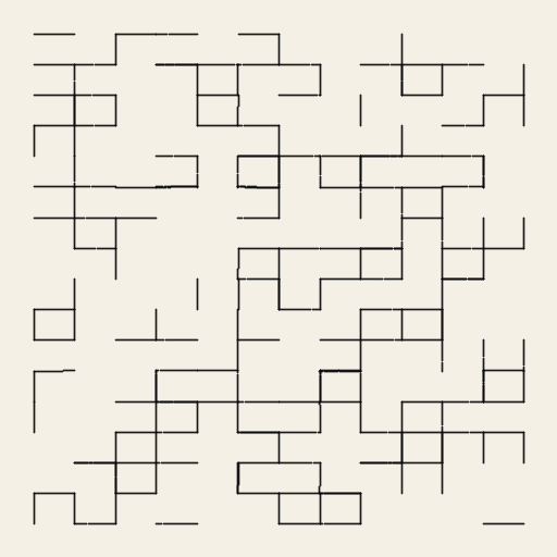
Vera Molnár's 1968 'Interruptions' series: a regular grid of rectangle cells where each cell's four border edges are drawn independently, each with its own random probability of being omitted.
Line Arrangements (Mohr)
generative_pioneers · mohr_line_arrangement
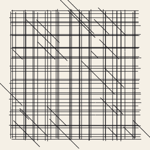
Manfred Mohr's 1969 plotter 'Line Arrangements': a fixed grid of columns and rows, each carrying a small set of nearly-parallel lines whose exact positions are random within the cell, overlaid with a layer of 45° diagonals whose length, position and orientation are independently random.
Plotter Trajectories (Hébert)
generative_pioneers · hebert_plotter_trajectory
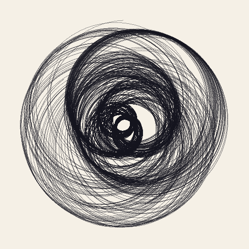
Jean-Pierre Hébert's plotter-trajectory idiom — parametric Lissajous-like curves drawn over multiple passes, each pass slightly phase-shifted, each segment modulated by the local velocity of the pen so that slow regions lay down heavier pigment and fast regions trace a ghost line.
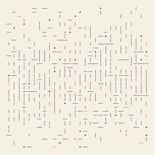
Walk-through-Raster (Nake)
generative_pioneers · nake_walk_sequence
Frieder Nake's 1966 'Walk-through-Raster' program (Algol 60 on a Telefunken TR4, plotted on a ZUSE Graphomat Z64): a repertoire of six signs — empty, vshort, vlong, hshort, hlong, dot — is sampled into a Markov chain whose transition probabilities vary with chain position so that 'vertical strokes are high at the chain's middle, empties dominate at the ends'.