generative_pioneers_2 · molnar_hypertransformations
Hypertransformations (Molnár)
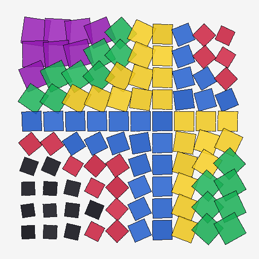
Vera Molnár's 'Hypertransformations' (1974-1976), executed on the IBM 360 with a CRT 2250 display and output on a Benson plotter. The work takes a regular grid of cells and, for each cell, applies a per-cell rotation, scale, displacement, and palette index derived from a continuous scalar field φ(u,v,t) = sin(kx·π·u + 0.6t) · cos(ky·π·v + 0.4t). The result is what Molnár called 'a vibrating force' acting on a regular orthogonal structure — the deformed grid is the visible trace of a parametric function the artist can tune step by step, then freeze as a single image. The signature Molnár tape ('75.058 15.06.04' / '15.07.51') records the exact moment each plotter drawing was completed, between 3:06.04 and 3:07.51pm on 27 February 1975.
Original: https://dam.org/museum/artists_ui/artists/molnar-vera/
▶ Try the live demo (JS port) ▶ Run reference.py via Pyodide 10 formulas have instant JS ports. The Pyodide path runs the actual Python in your browser — first load is ~6 MB, then instant.
Math essence
Each cell (ci, ri) is mapped to local coordinates (u, v) ∈ [0,1]²; a global field φ(u,v,t) = sin(kx·π·u + α·t)·cos(ky·π·v + β·t) drives rotation θ = amp_rot·φ, scale s = 1 + amp_scale·φ, displacement (dx, dy) = amp_disp·(φ, 1−φ), and a palette index ∝ φ. The deformation is continuous in (u, v, t) and renders as a quilt of tilted, scaled, recoloured squares.
Parameters
| Name | Type | Default | Range | Description |
|---|---|---|---|---|
dim | int | 512 | 200–1200 | Square canvas side length |
cols | int | 10 | 4–30 | Grid columns |
rows | int | 10 | 4–30 | Grid rows |
margin | float | 0.08 | 0–0.3 | Outer margin (fraction of dim) |
rotation_amp | float | 0.55 | 0–2 | Per-cell rotation amplitude (×π rad) |
displacement_amp | float | 0.18 | 0–0.6 | Per-cell translation amplitude (fraction of cell size) |
scale_amp | float | 0.35 | 0–0.8 | Per-cell scale modulation amplitude |
color_shift | float | 0.6 | 0–1.5 | Per-cell palette noise amplitude |
kx | float | 0.7 | 0–3 | x-frequency of the parametric field |
ky | float | 1.1 | 0–3 | y-frequency of the parametric field |
seed | int | null | 0–999999 | RNG seed |
Reference
First 60 lines of reference.py. Full source:
library_external/generative_pioneers_2/molnar_hypertransformations/reference.py
from __future__ import annotations

from typing import ClassVar

import imageio.v2 as imageio
import numpy as np


class MolnarHypertransformations:
    family: ClassVar[str] = "generative_pioneers_2"
    sketch: ClassVar[str] = "molnar_hypertransformations"

    def __init__(
        self,
        dim: int = 512,
        cols: int = 10,
        rows: int = 10,
        margin: float = 0.08,
        rotation_amp: float = 0.55,
        displacement_amp: float = 0.18,
        scale_amp: float = 0.35,
        color_shift: float = 0.6,
        kx: float = 0.7,
        ky: float = 1.1,
        seed: int | None = None,
    ) -> None:
        self.dim = dim
        self.cols = cols
        self.rows = rows
        self.margin = margin
        self.rotation_amp = rotation_amp
        self.displacement_amp = displacement_amp
        self.scale_amp = scale_amp
        self.color_shift = color_shift
        self.kx = kx
        self.ky = ky
        self._seed = seed
        self.rng = np.random.default_rng(seed)
        self.canvas = np.full((dim, dim, 3), 245, dtype=np.uint8)
        self.time = 0
        self._dirty = True

    def reset(self, seed: int | None = None) -> None:
        if seed is not None:
            self._seed = seed
        self.rng = np.random.default_rng(self._seed)
        self.canvas = np.full((self.dim, self.dim, 3), 245, dtype=np.uint8)
        self.time = 0
        self._dirty = True

    def _phi(self, u: float, v: float, t: float) -> float:
        return float(
            np.sin(self.kx * np.pi * u + 0.6 * t)
            * np.cos(self.ky * np.pi * v + 0.4 * t)
        )

    def _transformed_cell(
        self,
        cx: float,
        cy: float,
Try running it locally
The reference implementation is self-contained Python with numpy. Install the package and run:
python library_external/generative_pioneers_2/molnar_hypertransformations/reference.pyNeed help? See Learn for the standard environment setup, or Playground for an in-browser sketchbook.
More from generative_pioneers_2

Computer-Aided Painting (Schwartz)
generative_pioneers_2 · lillian_schwartz
Lillian Schwartz, who worked at Bell Labs from 1968 to 2001 with Kenneth C.
P-159 D (Mohr)
generative_pioneers_2 · mohr_p159d
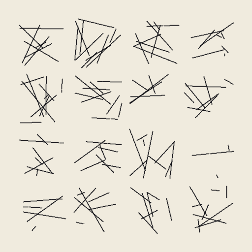
Manfred Mohr's 'P-159 D' (1969, Vincennes) sits in the P-159 family that the artist developed from his earlier P-021 / P-036 line-arrangement programs.
Raster Sequence (Nake)
generative_pioneers_2 · nake_raster_sequence
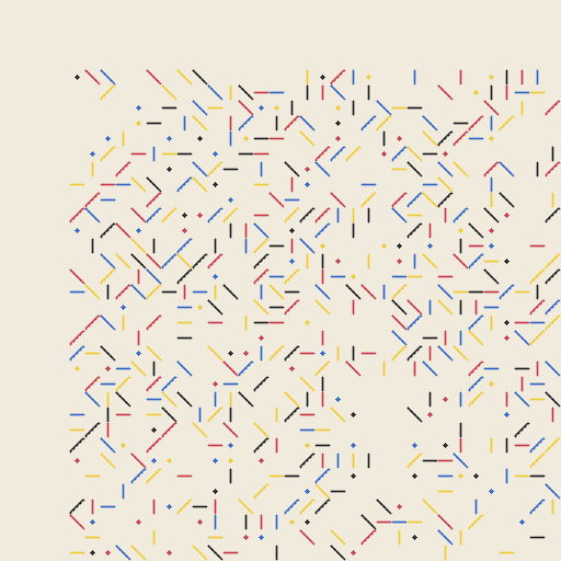
Frieder Nake's 'Walk-through-Raster' / 'Raster Sequence' (1966) is the first non-stationary Markov chain in computer art history.
Structure Computer (Cohen / AARON)
generative_pioneers_2 · cohen_structure_computer
Harold Cohen's AARON, begun at UCSD in 1967-1973 and continuously developed until Cohen's death in 2016, is the longest-running art-making AI in history.
Text Rain (Utterback & Achituv)
generative_pioneers_2 · utterback_text_rain
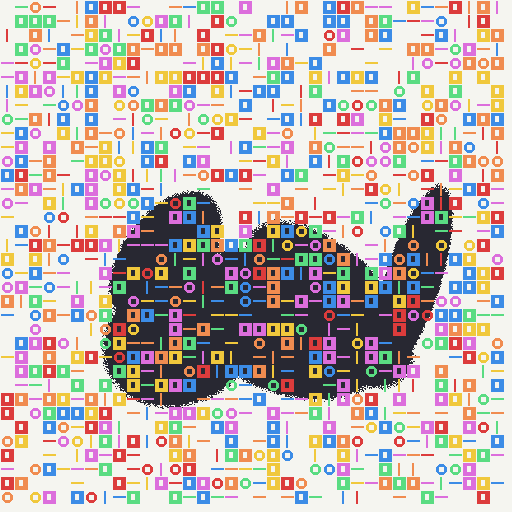
Camille Utterback and Romy Achituv's 'Text Rain' (1999) is one of the canonical interactive installations of the late-1990s computer-vision era, and the piece that won them a US patent (US 6,928,313) in 2005.
Wall Drawings (LeWitt)
generative_pioneers_2 · sol_lewitt_wall_drawings
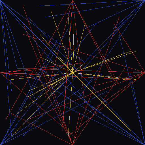
Sol LeWitt's wall drawings (1968-2007) are the canonical example of conceptual-art-as-algorithm: the work is the set of written instructions, and any number of draftspeople can execute them with different results that all satisfy the same rule.