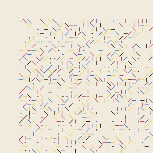
generative_pioneers_2 · nake_raster_sequence
Raster Sequence (Nake)
Frieder Nake's 'Walk-through-Raster' / 'Raster Sequence' (1966) is the first non-stationary Markov chain in computer art history. Programmed in Algol 60 on the Telefunken TR4 at Stuttgart, output on a ZUSE Graphomat Z64 flatbed, the algorithm has three parts: a fixed repertoire of six visual signs (empty, vertical stroke, horizontal stroke, both diagonals, dot), a first-sign selection function, and a non-stationary transition-probability matrix that slowly shifts the distribution of signs along the chain. The non-stationarity is the trick — at the beginning of the chain the empty sign dominates, then vertical strokes take over in the middle, and the empty sign returns at the end. The chain is then 'walked' through a fixed raster of cells, one sign per cell, in row-major order. Nake later added 'mapping modes' that re-order this walk (column-major, spiral, etc.). This reference uses six signs (matching the period notation), the same 'empty on the outside, vertical in the middle' bias, and row-major mapping as the default.
Original: https://dam.org/museum/wp-content/uploads/2021/05/FN_WalkThroughRaster.pdf
▶ Try the live demo (JS port) ▶ Run reference.py via Pyodide 10 formulas have instant JS ports. The Pyodide path runs the actual Python in your browser — first load is ~6 MB, then instant.
Math essence
A position-dependent 6×6 transition matrix T(pos) = T_base + bias(pos)·(T_centre − T_base), where bias(pos) = 1 − 4(pos − 0.5)², is used to draw a chain of length cols·rows from the six-sign alphabet. The chain is then placed into a cols×rows raster in row-major order. Increasing non_stationarity widens the difference between the centre and the ends of the chain, so the long vertical strokes cluster in the middle of the picture exactly as in Nake's original '7.3-1'.
Parameters
| Name | Type | Default | Range | Description |
|---|---|---|---|---|
dim | int | 512 | 200–1200 | Square canvas side length |
cols | int | 32 | 8–96 | Raster columns |
rows | int | 32 | 8–96 | Raster rows |
cell_size | int | 14 | 4–48 | Side length of one raster cell (px) |
margin | float | 0.06 | 0–0.3 | Outer margin (fraction of dim) |
non_stationarity | float | 0.7 | 0–1.5 | Strength of the centre/edge bias shift along the chain |
stochasticity | float | 1 | 0.2–2 | Temperature of the chain (lower = sharper peaks) |
bg_color | tuple | 240,235,220 | null–null | Background RGB |
ink_color | tuple | 12,14,22 | null–null | Ink RGB |
seed | int | null | 0–999999 | RNG seed |
Reference
First 60 lines of reference.py. Full source:
library_external/generative_pioneers_2/nake_raster_sequence/reference.py
from __future__ import annotations

from typing import ClassVar

import imageio.v2 as imageio
import numpy as np


class NakeRasterSequence:
    family: ClassVar[str] = "generative_pioneers_2"
    sketch: ClassVar[str] = "nake_raster_sequence"

    SIGN_EMPTY = 0
    SIGN_VERT = 1
    SIGN_HORIZ = 2
    SIGN_DIAG_R = 3
    SIGN_DIAG_L = 4
    SIGN_DOT = 5

    SIGNS = (
        "empty",
        "vertical",
        "horizontal",
        "diag_right",
        "diag_left",
        "dot",
    )

    BASE_TRANSITION = np.array(
        [
            [0.55, 0.10, 0.05, 0.10, 0.10, 0.10],
            [0.55, 0.20, 0.05, 0.10, 0.05, 0.05],
            [0.55, 0.05, 0.20, 0.05, 0.10, 0.05],
            [0.55, 0.10, 0.10, 0.15, 0.05, 0.05],
            [0.55, 0.05, 0.10, 0.05, 0.15, 0.10],
            [0.55, 0.10, 0.10, 0.10, 0.05, 0.10],
        ],
        dtype=np.float32,
    )

    def __init__(
        self,
        dim: int = 512,
        cols: int = 32,
        rows: int = 32,
        cell_size: int = 14,
        margin: float = 0.06,
        non_stationarity: float = 0.7,
        stochasticity: float = 1.0,
        bg_color: tuple[int, int, int] = (240, 235, 220),
        ink_color: tuple[int, int, int] = (12, 14, 22),
        palette: tuple[tuple[int, int, int], ...] = (
            (12, 14, 22),
            (200, 40, 60),
            (30, 90, 200),
            (240, 200, 40),
        ),
        seed: int | None = None,
    ) -> None:
        self.dim = dim
Try running it locally
The reference implementation is self-contained Python with numpy. Install the package and run:
python library_external/generative_pioneers_2/nake_raster_sequence/reference.pyNeed help? See Learn for the standard environment setup, or Playground for an in-browser sketchbook.
More from generative_pioneers_2
Computer-Aided Painting (Schwartz)
generative_pioneers_2 · lillian_schwartz
Lillian Schwartz, who worked at Bell Labs from 1968 to 2001 with Kenneth C.
Hypertransformations (Molnár)
generative_pioneers_2 · molnar_hypertransformations
Vera Molnár's 'Hypertransformations' (1974-1976), executed on the IBM 360 with a CRT 2250 display and output on a Benson plotter.
P-159 D (Mohr)
generative_pioneers_2 · mohr_p159d
Manfred Mohr's 'P-159 D' (1969, Vincennes) sits in the P-159 family that the artist developed from his earlier P-021 / P-036 line-arrangement programs.
Structure Computer (Cohen / AARON)
generative_pioneers_2 · cohen_structure_computer
Harold Cohen's AARON, begun at UCSD in 1967-1973 and continuously developed until Cohen's death in 2016, is the longest-running art-making AI in history.
Text Rain (Utterback & Achituv)
generative_pioneers_2 · utterback_text_rain
Camille Utterback and Romy Achituv's 'Text Rain' (1999) is one of the canonical interactive installations of the late-1990s computer-vision era, and the piece that won them a US patent (US 6,928,313) in 2005.
Wall Drawings (LeWitt)
generative_pioneers_2 · sol_lewitt_wall_drawings
Sol LeWitt's wall drawings (1968-2007) are the canonical example of conceptual-art-as-algorithm: the work is the set of written instructions, and any number of draftspeople can execute them with different results that all satisfy the same rule.